2.4 Reshaping data with pivot_longer()
2.4.1 Wide and long format
Let’s say you have some biological data (finally, wohoo!), and want to plot it using ggplot2. There are (at least) two ways your data can be formatted:
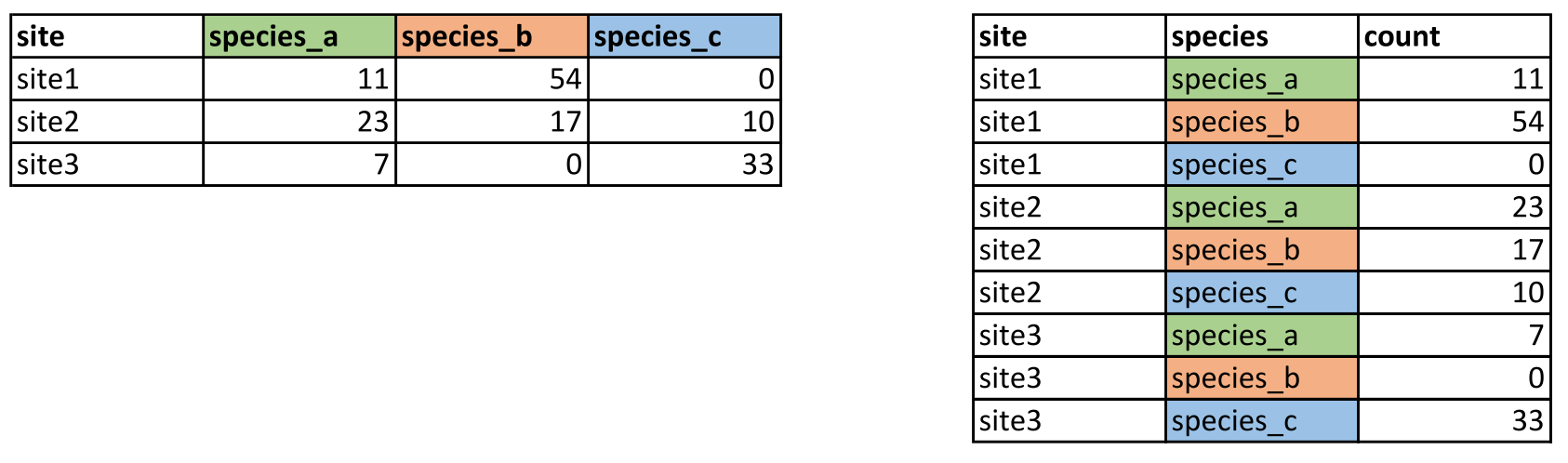
Figure 2.1: Data in “wide format” (left) and “long format” (right)
These two formats are commonly referred to as “wide” and “long” respectively. If you want to make some plot that is e.g. colored by species in this data, the data needs to be in long format, i.e. the variable you are grouping by has to be contained in a single column. Data can be converted from wide to long using the tidyverse function pivot_longer().
2.4.2 Import example data
Let’s import a data set to use as our example. Download copepods.txt here. The data contains counts of different copepod taxa from outside Drøbak.
Exercise: download the data and import it into R. Is this data “wide” or “long”?
Show hint
Use the read.table() function. The data is tabulator separated with a header. Remember to work in the correct working directory!
Take a look at the data and how it’s structured:
2.4.3 Reshape the data
As you hopefully figured out, this data is in so-called wide format, and we need to make it long with pivot_longer(). pivot_longer() has two important arguments called names_to and values_to. In our case names_to is the name of the new column of species, and values_to is the name of the new column where our values go. In addition, you need to provide the columns that you want to reshape. We can reshape this data like this:
copepods_long <- copepods %>%
  pivot_longer(c(acartia, calanus, harpacticoida, oithona, oncaea, temora),
               names_to = "species", values_to = "count")

copepods_long
#> # A tibble: 54 × 3
#>    depth species       count
#>    <int> <chr>         <int>
#>  1     0 acartia           0
#>  2     0 calanus           3
#>  3     0 harpacticoida     0
#>  4     0 oithona           2
#>  5     0 oncaea            0
#>  6     0 temora            0
#>  7     2 acartia           1
#>  8     2 calanus           0
#>  9     2 harpacticoida     0
#> 10     2 oithona           6
#> # ℹ 44 more rows
Note that pivot_longer() has the same way of selecting columns as select(), meaning we can use the minus sign to choose all columns except depth. The following code does the same as the one above:
That sure is more convenient than explicitly selecting all the columns we want (in our case, anyway)!
2.4.4 Plot the data
Now we can plot the data! By now, you should know enough ggplot to attempt this yourself.
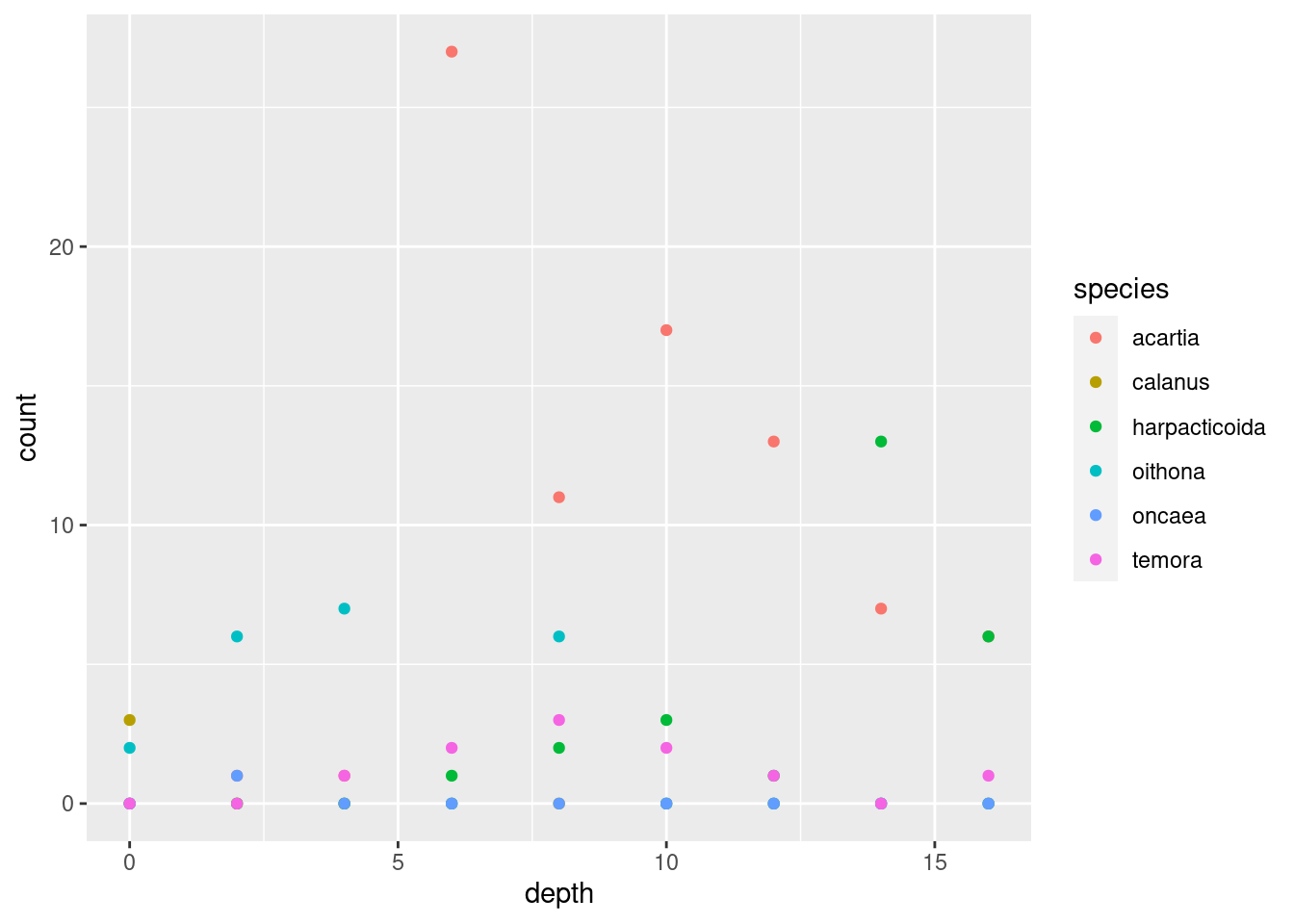
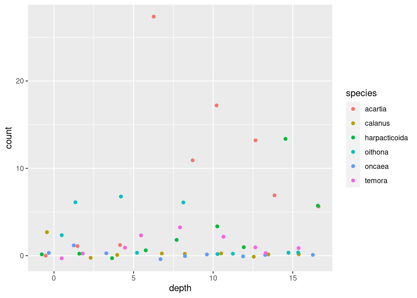
Exercise: Make a plot where you have depth on the x-axis and count on the y-axis, and color by species. Experiment with using some different geoms and find the most suitable for visualising your data. When you’ve settled on a geom, create a title and axis labels, and save your finished plot with ggsave()
Show some geom ideas
Try these, and see how they look for your data!
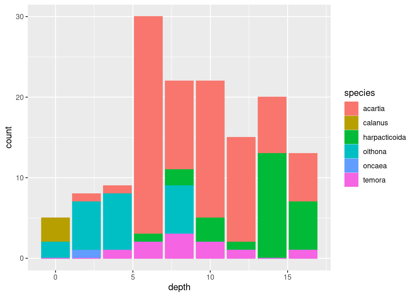
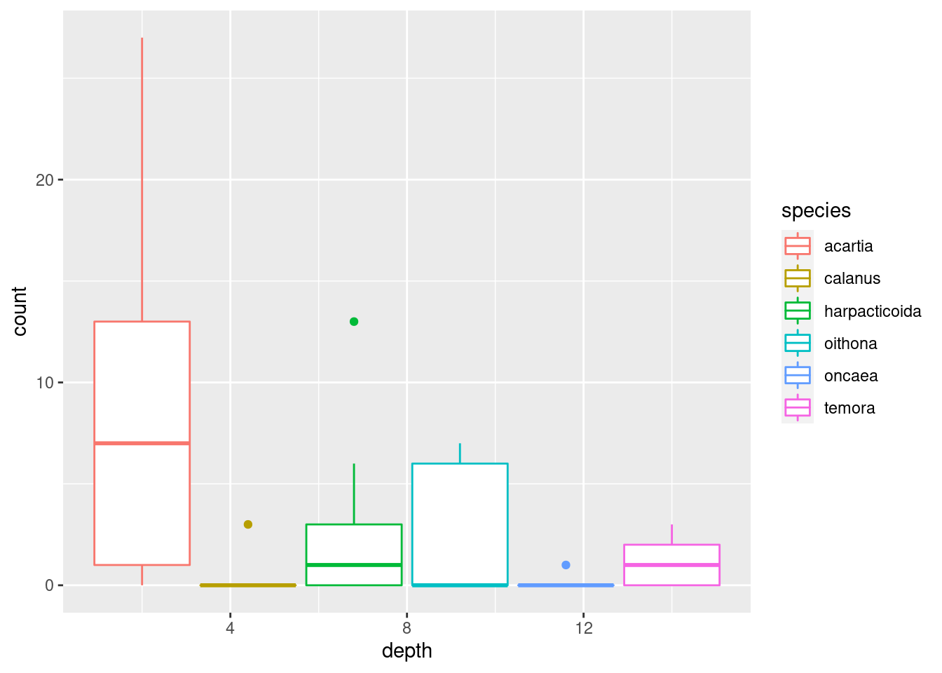
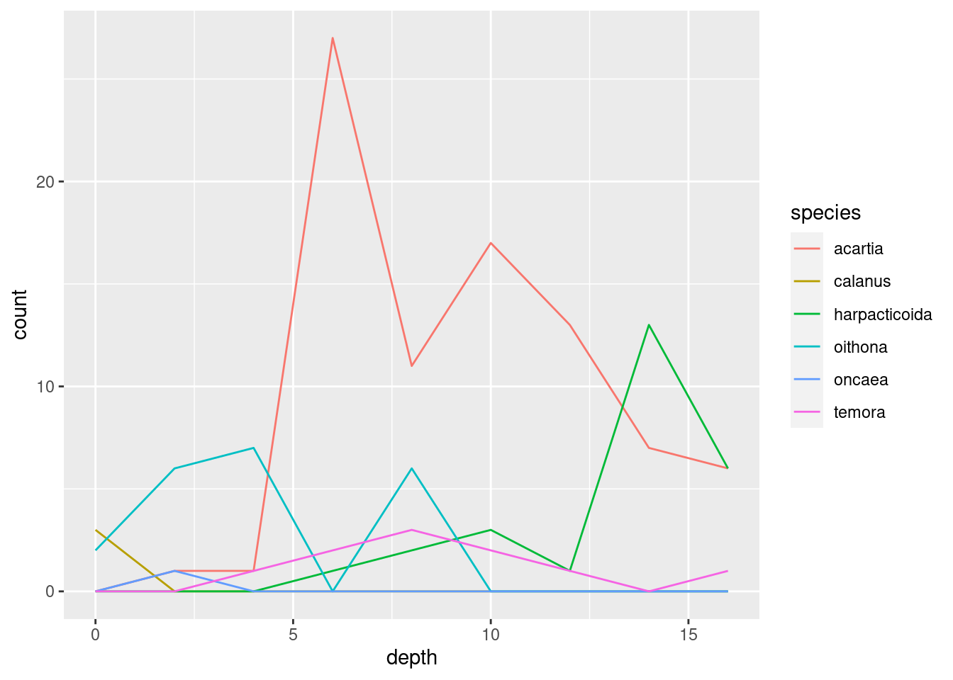
geom_point()geom_jitter()(what is the difference between this andgeom_point()?)geom_col()(tip: usefillaesthetic instead ofcol)geom_boxplot()(does this make sense?)geom_line()geom_area()(usefillfor this one too)
Show code and plots
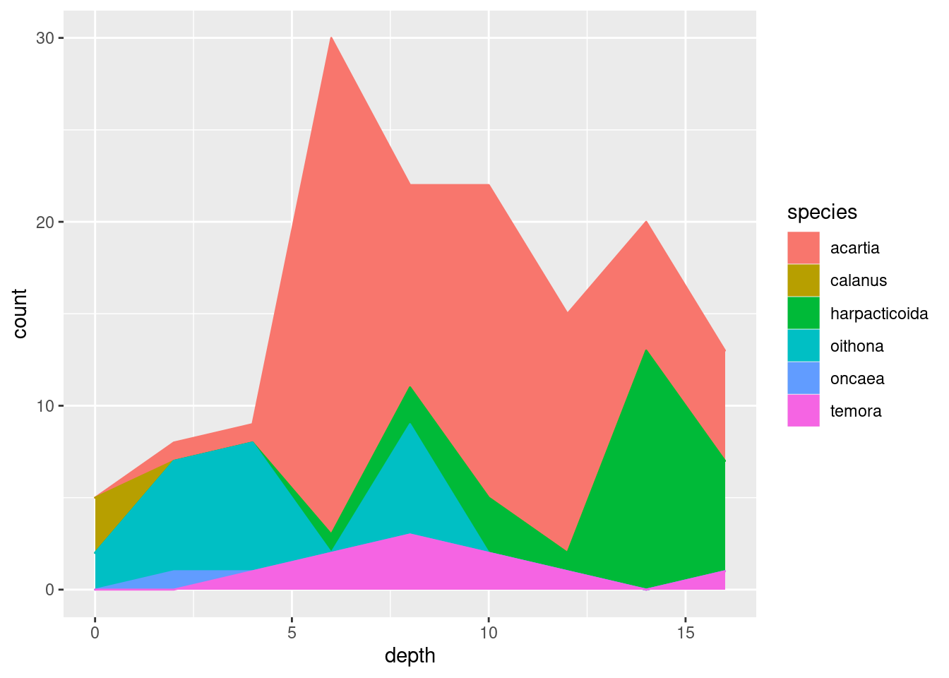
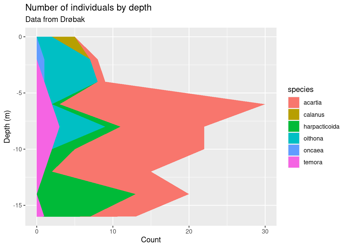
I’m settling on geom_area() since it nicely shows both total abundance and the relationship between the taxa (plus, it looks cool). Some additional tricks I do: flip the coordinates with coord_flip() to get depth on the y-axis, and plotting -depth instead of depth to plot depth downwards. I do this because it is how depth data is usually shown in marine biology, and because I wanted to show you that there are lots of options on customising plots that you will encounter as you learn more about ggplot.
copeplot <- ggplot(copepods_long, aes(-depth, count)) +
  geom_area(aes(fill = species)) +
  labs(title = "Number of individuals by depth",
       subtitle = "Data from Drøbak",
       x = "Depth (m)",
       y = "Count") +
  coord_flip()

copeplot